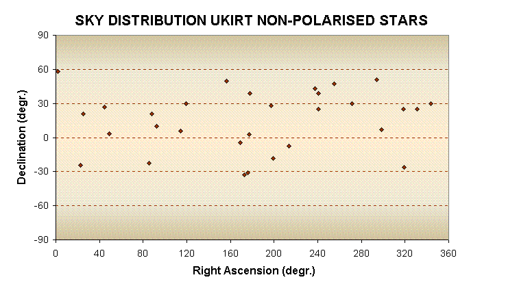
Figure 1: The distribution on the sky of UKIRT non-polarised stars. This distribution is relativity adequate over the part of the sky observable with the telescope (between declination +58 and -40).
SPECTROPOLARIMETRIC CALIBRATION
OF CanariCam: DEVELOPMENT OF A NETWORK OF CALIBRATION SOURCES FOR POLARIMETERS
ON LARGE TELESCOPES
Adapted from a paper presented
at the XII Canary Islands Winter School of Astrophysics
By Fabiola Martín-Luis
(CanariCam Calibration Team)
SUMMARY
When we do polarimetry, the presence of mirrors in the telescopes as well as the optics of the instruments which we use to carry out the polarimetric and spectropolarimetric measurements, introduce modifications in our observed polarisation that it is necessary to correct.
The main problem is that the instruments and the telescope introduce instrumental polarisation due to successive reflections of the beam after it is focused onto the detector. We must quantify that degree of polarisation and its orientation and, in addition, we need to check the efficiency of detection of polarisation from our sources.
Because of this, - as in photometry and spectrophotometry - we need calibrate our measurements by using standard stars. We need a network of objects with low polarisation (for the instrumental polarisation) and other stars with high degree of polarisation (for check the efficiency of detection).
At present, the most complete network of stars of low polarisation was elaborated in 1974 by Gehrels [1]. This list is used as the network of zero polarisation standards stars for UKIRT (United Kingdom InfraRed Telescope). However, this list - which is composed only for 30 stars - presents a low and inhomogeneous spatial density. Apart from this 50% of them are brighter than magnitude +5, and thus do not necessarily satisfy the flux requirements of the observers.
Our main goal is to find a network of suitable zero polarisation standards with high and homogeneous spatial density and with an adequate flux distribution. We have also carried out a study in which we compare the possibilities of using (i) a high polarisation object list or, (ii) an optical component which gives 100% polarisation. There are very few suitable high-polarisation stellar sources for calibration beyond 5 microns. The Serkowski Law suggests that no stars will be detectably polarised at 10 microns, although a few, very deeply embedded stars do have a degree of polarisation >5% at 10 microns. The simplest solution to the problem of checking the polarisation detection efficiency at the telescope however, is the insertion and retraction of a Glan prism.
This work aims to study the
polarimetric calibration of CC-Pol, the polarimetric module incorporated
in CanariCam - one of the 1 Day Instruments for the GTC - which will cover
the range from 8 to 24 microns. In addition, it is a part of the photometric,
spectrophotometric and polarimetric calibration for the CanariCam project.
THE PROBLEM
Instrumental polarisation
Instrumental polarisation is produced by reflections in the primary, second and tertiary mirrors of the telescope and by reflections in the instrument generally. For our polarimeter, CC-Pol, the biggest contribution is due to the tertiary mirror - Nasmyth -, which presents a reflection of 45 degrees. There are 9 reflections within the cryostat that contribute to the total instrumental polarisation. Although the internal instrument mirrors are very clean and reflective, the externals will not be controlled to such a degree: the instrumental polarisation is expected to increase as their reflectivity decreases.
CC-Pol will be used initially on the Nasmyth focus of the GTC, although it is expected that the instrument will later be mounted on the straight through Cassegrain focus, a distinct advantage for polarimetry. With a Cassegrain focus the instrumental polarisation (IP) from the telescope is negligible, with the induced linear polarisation for most telescopes usually ~0.05%.
Typically a 45 degree reflection, as occurs with a Nasmyth focus, will produce a linear polarisation of ~5% in the visible [2], 0.5% in the near-infrared [3], and less in the MIR, although the actual values depend on the nature of the reflecting surface and may change with time.
As long as any linear induced IP is small, it is added vectorially to the Stokes vector and can therefore be subtracted off in the same way. For other cases a full Mueller matrix treatment is needed.
The normal method of measuring polarisation efficiency is to use standard polarised stars or a standard calibrator. The latter is preferable as standard stars have generally low degrees of polarisation (~5% or less at V, and smaller at shorter and longer wavelengths), whereas calibrators are available which can produce polarisations of 100%. However, any calibrator may have to be after the Nasmyth mirror.
Introducing a highly polarised calibrator into the beam can also be a rapid way of checking that the polarimeter is operating correctly.
The polarisation PA is usually measured with respect to some instrumental zeropoint, which can depend on wavelength (e.g. the fast axis of a multi-element achromatic waveplate can vary by a few degrees over its useful wavelength range). This has to be converted to a reference direction on the celestial sphere. It is sufficient to use the polarisation efficiency calibrators to determine any wavelength dependence of PA for an instrument, and polarised standard stars to relate these PAs to the celestial sphere.
Polarised standards (see
[4] and references therein) are available for wavelengths between 0.3 and
2.5 microns, but at longer wavelengths the degrees of polarisation for
these stars are generally small. Stars embedded in dark clouds, with high
extinction, have been used for longer wavelengths [5] but there may be
some local polarisation produced by reflection nebulosity around the star,
and thus the polarisation may be aperture dependent, and may also be variable.
These issues are discussed in more detail later.
WHAT IS NEEDED
We need a list of high and low polarisation standard stars with:
ZERO POLARISATION STANDARDS
Low polarisation standards are essential for checking the instrumental polarisation and the zero point of the position angle. However, they are a trivial problem to resolve adequately.
As polarisation is almost always induced by the ISM and is rarely intrinsic to a star (except in very cool stars), any star in the solar neighbourhood should be unpolarised unless it is located in a region of particularly high density of the LISM. It is thus usually sufficient simply to select high proper motion stars and use these as zero polarisation stars.
A list of suitable non-polarised stars was given by Gehrels [1]. Most of these stars are type G dwarfs at high Galactic latitude with V magnitudes between +0.4 y +7.3. The range of magnitudes extends from V=+0.4 (Procyon), N=- 0.63, to V=7.3, N=5.7. The list of stars is available in the UKIRT pages at the URL: http://www.jach.hawaii.edu/JACpublic/UKIRT/instruments/ irpol/irpol_stds.html/#Unpolarized.
The sky coverage of the zero
polarisation stars is very uneven (see Figure 1). There is a hole in the
sky at high declinations that are not reachable from UKIRT. Therefore,
at very least time will be lost in moving the telescope between the source
and the calibration star. This issue is discussed below.
Figure 1: The distribution on the sky of UKIRT non-polarised stars. This distribution is relativity adequate over the part of the sky observable with the telescope (between declination +58 and -40).
There are only 30 stars in this list, and 13 of them (43%) are brighter than V=+5. This may lead to saturation problems even in polarimetric and imaging mode. The histogram of the magnitude distribution is shown in Figure 2.
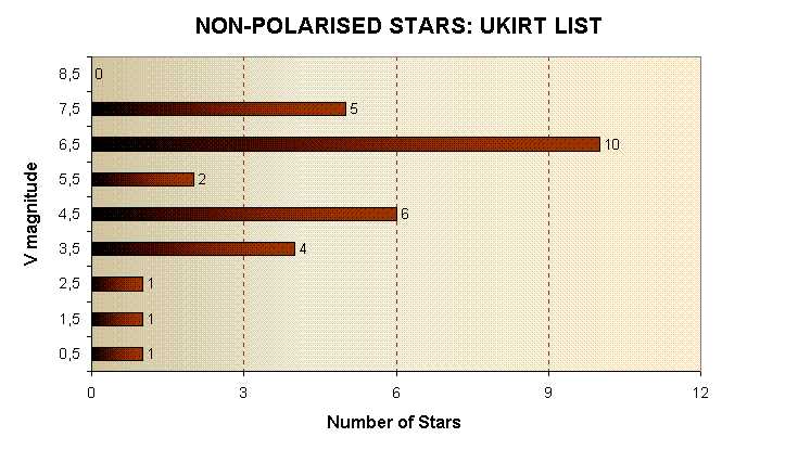
Figure 2: The distribution of brightness of UKIRT non-polarised stars by magnitude.
A better solution is to generate a new list of suitable stars.
Typically, the low polarisation stars present a low interstellar extinction. If a star is polarised it is probably produced due to ISM. Only in a few types of stars, the polarisation is intrinsic, e.g.: Wolf-Rayet stars, novae, planetary nebulae, red giants, etc.
The criterion that has been used is to select Main Sequence stars mainly within 100pc of the Sun, with a maximum extinction of 0.1 magnitudes in the visible and a spectral type no later than K3V. The aim was to obtain at least one star per 25 square degrees over the whole sky visible to the GTC, with a magnitude range suitable for the instrument (down to V~ 10, equivalent to N~ 8 for the faintest and reddest stars).
The search was made using a complete search of the SIMBAD database, selecting all stars within a given magnitude range and of a given spectral type. More than 25 000 stars were selected initially using these criteria. A posteriori, a careful selection of stars was made to eliminate all stars with an undesirable pathology (variability, peculiar spectral type, binarity, etc.). The next elimination criterion was by distance/extinction. A colour excess criterion was used to estimate the line of sight extinction. This is particularly important in the case of the rather more luminous (and thus distant) AV stars for which it was necessary to ensure that the line of sight extinction is low.
After those eliminations, a total of 3458 stars remained, with 2.75<V<10.90 and spectral type A0V - K3V. By spectral type, 602 stars (17.4%) were AV, 2151 (62.2%) were type FV, 691 (19.9%) were type GV, and 207 (5.4%) type KV.
These stars were then plotted on the sky to examine coverage. It was found that there is a heavy concentration of stars from - 10° > d > - 40°, presumably due to the sky coverage of the Michigan spectroscopic surveys. A further selection was thus made, by hand, to reduce the density of stars to as close to one star per 25 square degrees as possible. After removing stars that are in heavily over-sampled regions of the sky, 1156 stars remain that are, apart from certain small regions of the sky (mainly in the Galactic Plane) that are less well covered, well distributed.
In the last stage of the search, we checked the distances using Hipparcos data and non-local stars were eliminated. Thus, 651 stars remain.
The division of spectral types remains broadly unchanged after the thinning-out process. Of the 651 stars that were selected, slightly over 50% are of type FV. Overall: 71 (10.9%) are of type AV; 293 (45.0%) are of type FV; 175 (26.9%) are of type GV; and 112 (17.2%) of type KV.
The histogram of magnitudes for the final selection of stars is as shown in the Figures 3 & 4, as Johnson V and in broad-band N. Note that the most stars are 6<N<8. At N=8 we will obtain s/n>100 in 100 seconds given the expected sensitivity of the instrument, so we feel that this criterion is adequate.
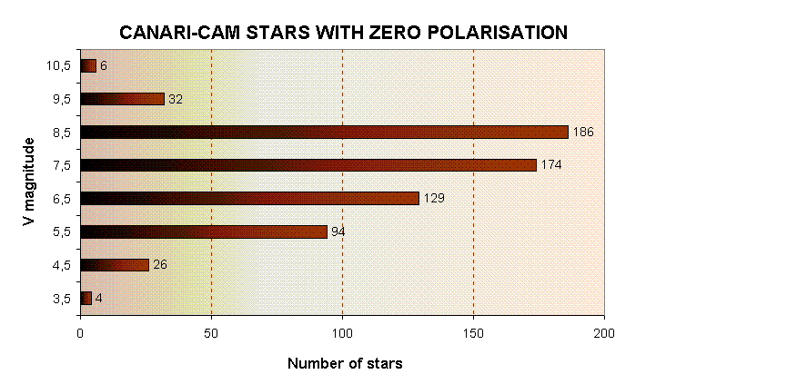
Figures 3 & 4: The distribution of brightness of CANARI-CAM non-polarised stars by V y N magnitudes. The maximum is between N=6 and N=7; for N=8, we will obtain s/n>100 in 100 seconds, so we feel that this criterion is adequate.
The corresponding distribution is:
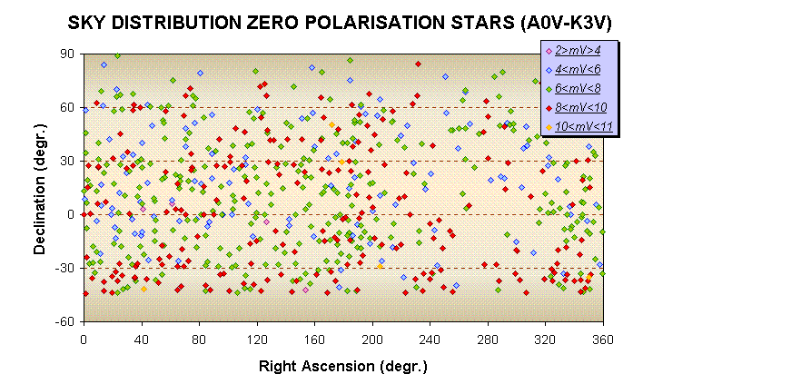
Figure 5: The distribution on the sky of CanariCam non-polarised stars by magnitude. Note that the spatial density decreases around the Galactic Centre because of the existence of dust.
We will need to check that the instrumental polarisation is constant during the night and does not depend of the telescope-instrument position (e.g. due to flexure). Therefore, an important part of the instrument's set-up and commissioning will be to observe zero polarisation stars in different points on the sky to check that the response is constant.
HIGH POLARISATION STANDARDS
High polarisation standards are useful for checking the efficiency of detection of the polarisation. In this case there are more serious and fundamental problems than for the zero polarisation stars. Although the polarisation detection efficiency can be measured easily in the laboratory (e.g. with a wire grid), it is convenient to check the polarisation efficiency at the telescope nightly using high polarisation stars. This enables potential instrumental problems to be identified and offers greater security to the user. These observations can be made in evening twilight as part of the standard instrumental set-up process.
Most stars are unpolarised intrinsically, although red giants do show a degree of intrinsic polarisation that can reach values greater than 10% [6]. However, these stars are not useful calibrators given that (i) the stars that show such large polarisations are Mira variables and show highly variable polarisation; and (ii) the polarisation shows a very strong FDP (Frequency Dependant Polarisation) with the peak value in the UV thus, at long wavelengths, the polarisation is likely to be very small.
Extrinsic polarisation comes from absorption within the LISM, thus the majority of high polarisation stars are highly reddened. The polarisation shows a strong frequency dependence, with a maximum usually in the visible, although it may be well to the red, and a drop into the near infrared. As such, even a star with 5-10% polarisation in I, will usually have a polarisation below 1% at 5 microns.
Many researchers have investigated the relationship between the observed polarisation at a given frequency and the frequency dependence of that polarisation degree. This allows, at least in theory, the polarisation degree to be calculated at any given wavelength given a single measured value.
Serkowski [7] found evidence of an empirical relationship between the polarisation measured at a particular wavelength and the maximum polarisation. This was later formalised in extensive studies by Coyne et al. [8] and by Serkowski et al. [9].
The Serkowski Law is given as:
Plambda = Pmax exp{- 1.15 ln2 (lambda max/lambda )}
Where:
Pmax is the maximum polarisation degree, which occurs at lambda max
And
Plambda is the degree of polarisation at any given wavelength lambda
If Pmax and lambda max are known we can calculate Plambda for any given wavelength. The value of lambdamax is found to be strongly correlated with the ratio of colour excesses such as EV- K/EB- V. (Serkowski et al.; [9]).
Later studies have shown that the Serkowski Law is an oversimplification. Although it can be expressed as a general law of the form:
Plambda = Pmax exp{- K ln2 (lambda max/lambda )}
The value of "K" is itself found to be a variable in studies by Wilking et al. [10] that combine visible and near-IR polarimetry, although Codina-Landaberry & Magalhaes [11] were the first to suggest that "K" is a variable. They find that a three-parameter fit is required with "K" itself a strong function of lambda max.
The conclusions of Wilking et al. were confirmed by Whittet et al. [4], although the exact for of the best fit to the data was slightly modified. They fit a relationship of the type:
K = a + blambda max
Although their best fit is consistent with a=0, hence:
Plambda = Pmax exp{- 1.86 lambda max ln2 (lambda max/lambda )}
A consequence of this relationship is that, as lambda max increases, the width of the polarisation curve decreases. Thus selecting a star with a large value of lambda max may not increase the expected polarisation at long wavelengths. It also implies that the degree of polarisation drops steeply at longer wavelengths, although many stars are found to be rather more strongly polarised in the near infrared than the Serkowski law would predict. Thus Serkowski standards are not suitable mid-infrared standard sources.
A graph of the function of Plambda against lambda for a wide range of values of lambda max, covering the entire observed range of observed values of lambda max is shown in Figure 6. A crossover point is observed at 5 microns after which it is the stars with the smallest wavelength for lambda max that have the highest polarisation.
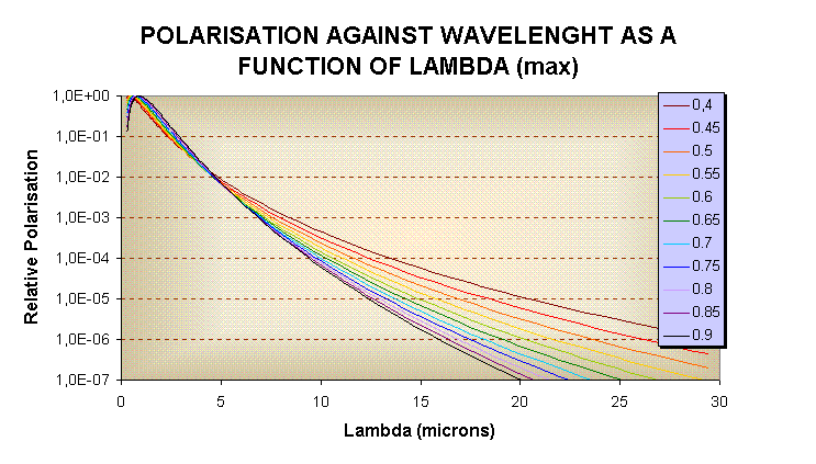
Figure
6: The expected polarisation as a function
of the peak polarisation and its wavelength for stellar source. Note that,
at 10 microns, the highest expected polarisations for stars are of the
order of 0.003 of the peak polarisation, i.e. for a star
that
is 10% polarised at peak, we expect < 0.03% polarisation at 10 microns.
Given that the best case has a polarisation at 10 microns that is just 0.3% of the peak value, in real astrophysical cases we expect only tiny polarisations to be found in stars. For a star that is 10% polarised at maximum, we can expect at most a polarisation of 0.03% at 10 microns - this is such a low value that it is of no practical use. At 20 microns the expected polarisations from stellar sources are 2-3 orders of magnitude lower still.
However, some deeply embedded objects though are polarised by as much as 15% at 10 microns and thus are potentially of great interest as calibrators for polarimetry. Smith et al. [5] present 8-13 microns spectropolarimetry of 55 sources and 16-22 microns spectropolarimetry of six of these. Almost all are objects at very low Galactic latitude. Most of the sources are embedded young stellar objects (YSOs), HII regions containing sites of star formation or bipolar protoplanetary nebulae (PPN), although a few other sources (e.g. NGC 1068, MWC 349) are also included. These represent a substantial fraction of all the star formation regions that can be observed in this way with current technology on 4-m class telescopes (i.e. brighter than about 20Jy at 10 microns in a 4-arcsec beam). The majority of the stars have oxygen-rich chemistry but there are three carbon-rich sources. Many of the oxygen-rich sources show deep silicate absorption overlying featureless, or optically thin silicate emission.
The data quality for the sources is highly variable. Some objects have errors of 0.1% or less, whilst the errors on the fainter sources may be greater than 1%. However, a significant fraction of the sources are well enough observed that they are suitable calibration sources for checking the efficiency of polarisation detection on the sky. Note though that careful source selection will be required as some of the objects have an extended polarisation component from surrounding nebulosity. These objects will be clearly resolved with CC-Pol due to its diffraction-limited imaging capability and thus are not suitable for calibration purposes.
The sky distribution of this list of high polarisation objects is presented in the Figure 7, and Figure 8 represents the sky distribution of those objects in function of their errors.
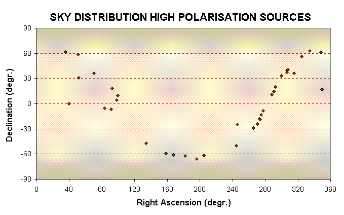
Figure 7: The sky distribution of high polarisation sources. The sources are distributed around the Galactic Plane where the dust is more abundant. [The red line indicates the GTC horizon].
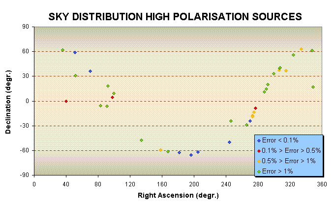
Figure 8: The sky distribution of high polarisation sources by data quality. The distribution of the most precisely measured sources (blue dots) is rather poor and few are available above the GTC horizon.
Note that the sources are relatively evenly distributed around the Galactic Plane. In some fields there are several objects that superimpose on the plot. However, the distribution of the most precisely measured sources (errors <0.5% in the total polarisation) is rather poor, with only six well-measured sources being available above the GTC horizon. This will severely limit their effectiveness as calibration sources for CC-Pol on the GTC. Furthermore, there is another problem: many of the nearby polarised sources are extended and the more distant ones are highly variable, in both cases making them unsuitable.
But there is another possible solution: we can use an instrumental method - for problem of checking the efficiency of polarisation detection. A simple solution is to switch a polariser into the beam that generates 100% polarisation (e.g. a polaroid sheet). A single measurement per night is sufficient to validate the instrumental performance in normal conditions, this measurement could be made as part of the normal instrumental set-up before observing each night.
The simplest solution to
the problem of checking the detection efficiency of polarisation is thus
to arrange to switch a Glan prism into the beam. This allows a measurement
to be made with a 100% polarised beam. The instrumental stability will
be such that a single measurement with this configuration at the start
of observations should be sufficient in all normal cases. This solution
is probably preferable to an astronomical calibration. But, we need to
be sure that the efficiency is constant during the night. Therefore, if
we have any object with a high degree of polarisation, we will increase
the reliability of our calibration capability.
FUTURE WORK
First, we plan to check the
initial network of low polarisation stars. We will make a new selection
by using a position criterion. Then, we will carry out polarimetric observations
of the list of low polarisation stars in order to obtain their polarisation
degree and position angle. We need a high degree of accuracy in the observations
of the standards stars because we want an effective calibration. At present,
we plan to observe in the NOT (Nordic Telescope; Observatorio del Roque
de los Muchachos. La Palma). Stars that are found to be zero polarised
in the visible can be safely assumed to be totally non-polarised in the
infrared; any star that is found to be significantly polarised is however
likely to be anomalous and will be rejected as a potential calibration
source.
BIBLIOGRAPHY
[2] 1960: Gehrels, T. "Instrumental Polarisation". AJ, 65, 466.
[3] 1971: Dyck, H. M. et al. "Polarimetry of red and infrared stars,at 1 to 4 microns". AJ, 76, 901.
[4] 1992: Whittet et al. "Systematic variations in the wavelength dependence of interstellar linear polarisation". ApJ, 386,562.
[5] 2000: Smith et al. "Studies in mid-infrared spectropolarimetric - II. An atlas of spectra". MNRAS, 312, 327.
[6] 1968: Kruszewski et al. "Wavelength dependence of polarisation. XII. Red variables". AJ, 73, 677.
[7] 1968: Serkowski, K. "Correlation Between the Regional Variations in Wavelength Dependence of Interstellar Extinction and Polarisation". ApJ, 154, 115.
[8] 1974: Coyne et al. "Wavelength dependence of polarisation. XXVI. The wavelength of maximum polarisation as a characteristic parameter of interstellar grains". AJ, 79, 581.
[9] 1975: Serkowski et al. "Wavelength dependence of interstellar polarisation and ratio of total to selective extinction". ApJ, 196, 261.
[10] 1980: Wilking et al. "The wavelength dependence of interstellar linear polarisation". ApJ, 235, 905.
[11] 1976: Codina-Landaberry et al. "On the polarizing interstellar dust". A&A, 49, 407.